Blogs On Programming

In this blog, we will discuss the Tree as a part of Graphs, as well as Tree traversal algorithms and Special types of trees. The tree data structure is used to present a hierarchical relationship between the data. The elements of the tree are called nodes. Starting from the root (initial) node, each node has a certain number of children. The nodes higher in the hierarchy are called the parent nodes and the children are called the child nodes. The nodes having the same parent are called siblings. The node with no child node is called a leaf node. The level of a node is the depth of the tree from that node to the root node. Since the tree is a hierarchical structure, the child node at one level can act as the parent node for the nodes at the next level. The tree in which each node has a maximum of 2 child nodes is called a Binary tree. Nodes of a binary tree can be represented using a structure or a class consisting of node information and a pointer each for the left and the right child node. The process of accessing the elements of a tree is called tree traversal. There are 4 types of tree traversal algorithms: 1. Inorder traversal: For Inorder traversal, the left subtree of a node is accessed first followed by the value of the node and then the right subtree of the node. For example, consider the following tree.     The Inorder traversal of the tree in Fig 1 will be 8,4,9,2,10,5,11,1,12,6,13,3,14,7,15. 2. Preorder traversal: For Preorder traversal, the value of the node is accessed first followed by the left subtree of a node and then the right subtree of the node. The Preorder traversal of the tree in Fig 1 will be 1,2,4,8,8,5,10,11,3,6,12,13,7,14,15. 3. Postorder traversal: For Postorder traversal, the left subtree of the node is accessed first followed by the right subtree of a node, and then the value of the node. The Postorder traversal of the tree in Fig 1 will be 8,9,4,10,11,5,12,13,6,14,15,7,3,1.  4. Level order traversal: For Level order traversal, starting from the root node, the nodes at a single level are accessed first before moving to the next level. Level order traversal is also Breadth-first traversal (BSF). The Level order traversal of the tree in Fig 1 will be 1,2,3,4,5,6,7,8,9,10,11,12,13,14,15. Binary Search Tree can also be converted to a doubly linked list such that the nodes of the doubly linked list are placed according to the inorder traversal of the tree. Special types of trees: 1. Binary Search Trees: A Binary search tree (BST) is a special type of tree in which the nodes are sorted according to the Inorder traversal. The search time complexity in a binary tree is O(log n). Insertion in a BST is achieved by moving to the left subtree if the value of the node to be inserted is lower than the current node or by moving to the right subtree if the value of the node to be inserted is greater than the current node. This process is repeated until a leaf node is found. 2. AVL Trees: AVL trees are BSTs in which for each node, the difference between the max level of the left subtree and the max level of the right subtree is not more than 1. AVL trees are also called the self-balancing BSTs. 3. Red Black Trees: Red Black trees are BSTs in which the nodes are colored either black or red with the root node always being black. No adjacent nodes in a Red Black tree can be red and for each node, any path to a leaf node has the same number of black nodes. Like AVL trees, Red Black trees are also self-balancing BSTs. 4. Trie: Trie is a special type of independent data structure which is in the form of a tree. It is generally used for string processing. Each node in a Trie has 26 child nodes indicating one of 26 English characters. Trie also has a Boolean data element marking the end of a string. The structure of a Trie can differ to incorporate various use cases. 5. Threaded Binary Trees: Threaded binary trees are used to make an iterative algorithm for the inorder traversal of a tree. The idea is to point the null right child of any node to its inorder successor. There are two types of threaded binary trees. a. Single-threaded: Only the right null child of each node points towards the inorder successor of the tree. b. Double-threaded: Both the left and the right null child of each node point towards the inorder predecessor and inorder successor of the node respectively. 6. Expression Trees: An Expression tree is a special type of tree used to solve mathematical expressions. Each non-leaf node in an expression tree represents an operator and each leaf node is an operand.   Ending note: In this blog, we discussed the Tree in data structures and Tree Transversal Algorithms used in Machine learning. Special trees help to solve different problems in optimized time and space. Overall, trees are advantageous as they depict a structural correlation between the data. Moreover, trees also provide flexible insertion and sorting advantages. Get one step closer to your dream job! Check out the books we have, which are designed to help you clear your interview with flying colors, no matter which field you are in. These include HR Interview Questions You’ll Most Likely Be Asked (Third Edition) and Innovative Interview Questions You’ll Most Likely Be Asked.

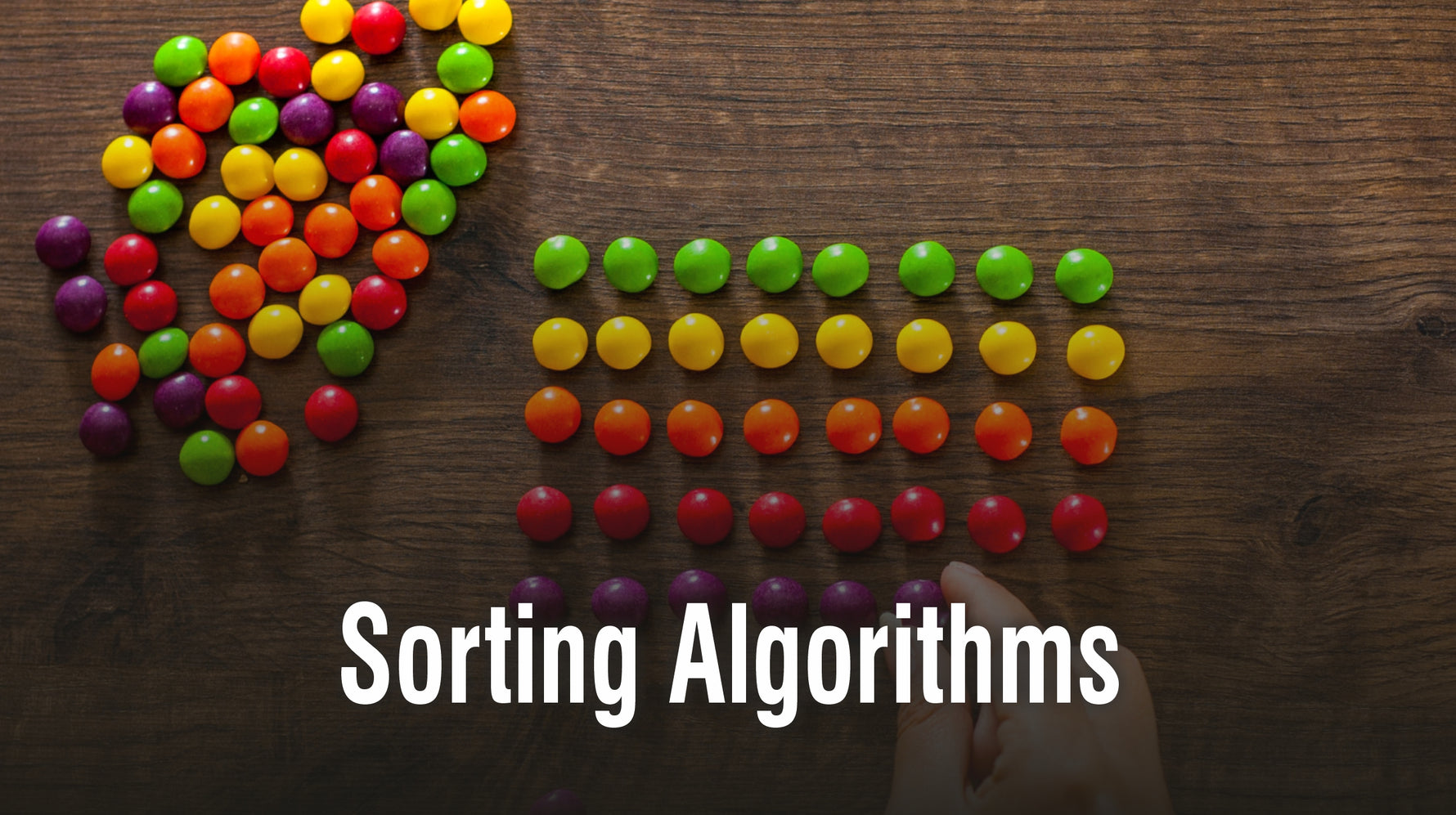
Algorithms are sequenced steps of instructions proposing a generalized solution for a problem. Algorithms determine the efficiency of a coding solution. They are divided into different categories depending on their nature of implementation. In this blog, we will discuss Sorting Algorithms focusing on their description, the way they work, and some common implementations.     Sorting Algorithm: As the name describes, the sorting algorithm is generally used to sort an array in a particular order. An array sorted in an ascending order means that every successor element in an array is greater than the previous one. A sorting algorithm takes an array as an input, performs sorting operations on it, and outputs a permutation of the array that is now sorted. Array {a, b, c, d} is alphabetically sorted. Array {1, 2, 3, 4} is sorted in ascending order. Generally, sorting algorithms are divided into two types: Comparison Sort and Integer Sort.   Comparison Sort: Comparison sort algorithms compare elements at each step to determine their position in the array. Such algorithms are easy to implement but are slower. They are bounded by O(nlogn), which means on average, comparison sorts cannot be faster than O(nlogn).     Integer Sort: Integer sort algorithms are also known as counting algorithms. The integer sort algorithm checks for each element, say x, how many elements are smaller than x and places x at that location in an array. For element x, if 10 elements are less than x then the position of element x is at index 11. Such algorithms do not perform comparisons and are thus not bound by Ω (nlogn). The efficiency of the selected sorting algorithm is determined by its run time complexity and space complexity.   Stability of a Sorting Algorithm: A sorting algorithm is said to be stable if it preserves the order of the same or equal keys in the output array as it is in the input array. Keys are the values based on which algorithm is sorting an array. Below is an example of stable sorting, Following is an unstable sorting as the order of equal keys is not preserved in the output. Next, let’s discuss some commonly used sorting algorithms.   Insertion Sort: This is a comparison-based algorithm. It takes one element, finds its place in the array, places it there, and in doing so sorts the whole array. For an array of size n, insertion sort considers the first element on the left as a sorted array and all the remaining n-1 elements on the right as an unsorted array. It then picks the first unsorted element (element number 2 of the array) and places it with a sorted element on the left moving elements if necessary. Now there are two arrays, a sorted array of size 2 and an unsorted of size n-2. The process continues until we get the whole array sorted, starting from the left. The best case of insertion sort is O(N) and the worst-case O(N^2).     Selection Sort: Selection sort is quite an easy algorithm in terms of implementation. It selects the smallest element present in an array and replaces it with the first element. It again scans for the smallest element in the remaining n-1 array and replaces it with the second element or the first element of the unsorted (n-1) array. The process of selecting the smallest element and replacing it continues until the whole array is sorted. The selection sort algorithm has the best and worst-case of O(N^2).     Merge Sort: Merge is a comparison-based algorithm that works on merging two sorted arrays. The technique used by the merge sort is divide and conquer. It divides the array into two subarrays, performs sorting on them separately, either recursively or iteratively, and then merges these two sorted subarrays. The result is a sorted array. Merge sort works in O(nlogn) run time.     Heap Sort: The comparison-based heap sort algorithm uses a binary heap data structure for sorting an array. A max-heap is formed from an unsorted array. The largest element from the binary heap is selected. As it is max-heap, the root is the largest value. This maximum value is placed at the end of an array. The heap shrinks by 1 element and the array increases by 1 element. Again, the above process is applied to the remaining heap. That is, convert it into max-heap and then replace the root (maximum) element with the last element. The process is repeated till we get a sorted array and the heap is shrunk to 0 elements. The run time of heap sort is O(nlogn).     Quick Sort: Quicksort works on the divide and conquer strategy. It selects a pivot element and forms two subarrays around this pivot. Suppose the pivot element is A[y]. Two subarrays are sorted as A[x,… y-1] and A[y+1,… z] such that all elements less than the pivot are in one subarray, and all elements greater than the pivot are in the second subarray. The subarrays can be sorted recursively or iteratively. The outcome is a sorted array. The average run time complexity of a quick sort is O(nlogn).     Bubble Sort: This comparison-based sorting algorithm compares elements of an array in pairs. The algorithm ‘bubbles’ through the entire array from left to right, considering two elements at a time and swapping the greater element with the smaller element of the pair. For an array A, element A[0] is compared with element A[1]. If element A[0] > A[1], they are swapped. Next, elements A[1] and A[2] are compared and swapped if required. These two steps are repeated for an entire array. The average run time complexity of Bubble sort is O(n2) and is considered an inefficient algorithm.     Shell Sort: Shell sort algorithm, in a way, works on insertion sort. It is considered faster than the insertion sort itself. It starts by sorting subsets of the entire array. Gradually the size of subarrays is increased till we get a complete sorted array as a result. In other words, shell sort partially sorts the array elements and then applies insertion sort on the entire array.   Shell sort is generally optimized using different methods to increase the size of subsets. The most commonly used method is Knuth’s method. The worst case of shell run time is O(n^(3/2) using Knuth’s method.     Distribution Sort Algorithms: Sorting algorithms where input is distributed into substructure, sorted, and then combined at the output are distribution sort algorithms. Many merge sort algorithms are distribution sort algorithms. Radix sort is an example of distribution sorting. Counting Sort: Counting sort is an integer-based sorting algorithm instead of a comparison-based sorting algorithm. The algorithm works on the assumption that every element in the input list has a key value ranging from 0 to k, where k is an integer. For each element, the algorithm determines all the elements that are smaller than it, and in this way places that element at an appropriate location in the output list. For this, the algorithm maintains three lists – one as an input list, the second as a temporary list for key values, and the third as an output list. Counting sort is considered as an efficient sorting algorithm with a run time of Θ(n) where the size of the input list, n, is not much smaller than the largest key value of the input list, k.   Radix Sort: Radix sort works on the subarrays and uses the counting sort algorithm to sort them. It groups the individual keys that take the same place and value. It sorts from the least significant digit to the most significant digit. In base ten, radix sort will first sort digits in 1’s place, then at 10’s place, and so on. The sorting is done using the counting sort algorithm. Counting sort can sort elements in one place value. As an example, base 10, can sort from 0 to 9. For 2-digit numbers, it will have to deal with base 100. Radix sort, on the other hand, can handle multi-digit numbers without dealing with a large range of keys. The list [46, 23, 51, 59] will be sorted as [51, 23, 46, 59] as for 1’s place value 1<3<6<9. Sorting of second place value will give [23, 46, 51, 58]. Another important property of the radix sort is its stability. It is a stable sorting algorithm. The runtime of radix sort is O(n) which means it takes a linear time for sorting.   Ending Note: Sorting algorithms are quite important in computer science as they help in reducing the complexity of the problem. The sorting algorithms that we discussed above have useful applications in databases, search algorithms, data structure, and many other fields of computer science.     Get one step closer to your dream job! Prepare for your interview by supplementing your technical knowledge. Our Job Interview Questions Book Series is designed for this very purpose, aiming to prepare you for HR questions you’ll most likely be asked. Check out the book here! panels.

Searching algorithms belong to a category of widely used algorithms in Computer Science. Searching algorithms are mainly used to lookup an entry from data structures, such as linked lists, trees, graphs, etc. In this blog, we will discuss the working, types, and a few implementations of searching algorithms. Searching Algorithm: A searching algorithm is used to locate and retrieve an element – say x – from a data structure where it is stored – say a list. The algorithm returns the location of the searched element or indicates if it is not present in the data structure. Searching algorithms are categorized into two types depending upon their search strategy. Sequential Search: These algorithms linearly search the whole data structure by visiting every element. These algorithms are, therefore, comparatively slower. An example is a linear search algorithm. Interval Search: these algorithms perform searching in a sorted data structure. The idea is to target the center of the data structure and then perform a search operation on the two halves. These algorithms are efficient. An example is a binary search algorithm. Next, let’s discuss some commonly used searching algorithms. Linear Search: The very basic searching algorithm traverses the data structure sequentially. The algorithm visits every element one by one until the match is found. If the element is not present in the data structure, -1 is returned. Linear search applies to both sorted and unsorted data structures. Although the implementation is quite easy, linear search has a time complexity of O(n), where n is the size of the data structure. It means it is linearly dependent on the size and quite slow in terms of efficiency. Binary Search: Binary search works on a sorted data structure. It finds the middle of the list. If the middle element is the required element, it is returned as a result. Otherwise, it is compared with the required element. If the middle element is smaller than the required element, the right half is considered for further search, else the left half is considered. Again, the middle of the selected half is selected and compared with the required value. The process is repeated until the required value is found. Binary search with time complexity of O(nlogn) is an efficient search algorithm, especially for large and sorted data records. Interpolation Search: Interpolation search is a combination of binary and linear search algorithms. Also called an extrapolation search, this algorithm first divides the data structure into two halves (like binary search) and then sequentially searches in the required half (linear search). In this way, it saves from dividing the data structure into two halves every time as in a binary search. For an array, arr[], x is the element to be searched. The ‘start’ is the starting index of the array and ‘end’ is the last index. The position of the element x is calculated by the formula: position = start + [ (x-arr[start])*(end-start) / (arr[end]-list[start]) ] The position is calculated and returned if it is a match. If the result is less than the required element, the position in the left sub-array is calculated. Else, the position is calculated in the right sub-array. The process is repeated until the element is found or the array reduces to zero. Interpolation search works when the data structure is sorted. When the elements are evenly distributed, the average run time of interpolation search is O(log(log(n))). Breadth-First Search Algorithm: BFS is used to search for a value in a graph or tree data structure. It is a recursive algorithm and traverses the vertices to reach the required value. The algorithm maintains two lists of visited vertices and non-visited vertices. It is implemented using a queue data structure. The idea is to visit every node at one level (breadth-wise) before moving to the next level of the graph. The algorithm selects the first element from the queue and adds it to the visited list. All the adjacent vertices (neighbors) of this element are traversed. If a neighbor is not present in the visited list, it means it is not traversed yet. It is placed at the back of the queue and in the visited list. If a neighbor is present in the visited list already, it means it has been traversed and is ignored. The process is repeated until the required element is found or the queue is empty. The following example will make the concept clear of breadth-first traversal.       Depth First Search Algorithm: This is another recursive search algorithm used for graphs and trees. In contrast to the BFS algorithm, DFS works on the strategy of backtracking. The algorithm keeps on moving to the next levels (depth-wise) until there are no more nodes. The algorithm then backtracks to the upper level and repeats for the other node. The DFS algorithm is implemented using a stack data structure. The algorithm pops an element from the top of the stack and places it in the visited list. All the nodes adjacent to this element are also selected. If any adjacent node value is not present in the visited list, it means it is not traversed yet, and it is placed at the stack top. Steps are repeated until the element is found or the stack is empty. See the following example for a better understanding of depth-first traversal.       Next, let’s discuss some common algorithm solutions for searching problems. Problem 1: Find the largest element in an array of unique elements. Algorithm: We can use Linear Search to find the largest element in an array of size n. The time complexity would be O(n). Initialize an integer value as max = 0. In a loop, visit each element in an array and compare it with the max value. If the element is greater than the max, swap it with the max value. When the loop ends, the max will contain the largest element of the array. Problem 2: Find the position of an element in an infinite sorted array Algorithm: A sorted array indicates that a binary search algorithm can work here. Another point to note is that the array is infinite. It means we don’t know the maximum index or upper bound of the array. To solve such a problem, we will first find the upper index and then apply the binary algorithm on the array. To find the upper bound/index of the infinite array: Initialize integer min, max, and value for minimum, maximum, and first array element. Set min, max, and value as 0, 1, and arr[0]. Run a loop until the value is less than the element we are looking for. If the value is less than the element swap min with the max, double the max, and store arr[max] in value. At the end of the loop, we get lower and upper bounds of the array in min and max. We can call binary search on these values. For binary search: If the max value is greater than 1, find mid of the array by min + (max -1)/2. If mid is the value we are looking for, return mid. If mid is less than the search value, call binary search on the left half of the array. Take mid-1 as the maximum bound. Else, call binary search on the right half of the array, and take mid+1 as the minimum bound.   Problem 3: Find the number of occurrence for an element in a sorted array Algorithm: To find how many times the element appears in a sorted array, we can use both linear and binary search. In linear search, maintain two integer variables result and key. Loop over the entire array, on every occurrence of the key, increment the result by 1. At the end of the loop, the result contains the number of occurrences of the key. Problem 4: Find if the given array is a subset of another array: Algorithm: For this problem, we don’t know if the array is sorted or not. The algorithm for linear search includes running two loops for array 1 and array 2. The outer loop selects elements of array 2 one by one. The inner loop performs a linear search in array 1 for array 2’s element. The complexity of this algorithm is O(mxn), where m and n are the sizes of array 1 and array 2, respectively. The problem can also be solved using binary search after sorting the array. First sort array 1. The time complexity of sorting is O(m log m). For each element of array 2, call binary search on array 1. Time complexity is O(n log m). The total time complexity for the algorithm is O(m logm + n logm), where m and n are the sizes of arrays 1 and 2, respectively. Ending Note: In this blog on searching algorithms, we discussed a very basic algorithm type. Search algorithms are the most commonly used algorithms, as the concept of searching data and records is quite common in software development. The records from databases, servers, files, and other storage locations are searched and retrieved frequently. Efficient searching algorithms with efficient time and storage complexity play a key role here. Get one step closer to your dream job!   Prepare for your programming interview with Data Structures & Algorithms Interview Questions You’ll Most Likely Be Asked. This book has a whopping 200 technical interview questions on lists, queues, stacks, and algorithms and 77 behavioral interview questions crafted by industry experts and interviewers from various interview panels.

The concept of data compression is very common in computer applications. Information is transmitted as a bit-stream of 0’s and 1’s over the network. The goal is to transmit information over the network with a minimum number of bits. Such transmission is faster in terms of speed and bandwidth. Huffman Coding is one such technique of data compression. This blog discusses Huffman coding, how it works, its implementation, and some applications of the method.   What is Huffman Coding? This data compression method assigns codes to unique pieces of data for transmission. The data byte occurring most often is assigned a shorter code whereas the next most occurring byte is assigned a longer code. In this way, the whole data is encoded into bytes. The two types of encoding methods used by Huffman coding are Static Huffman encoding and Dynamic Huffman encoding. Static Huffman encoding encodes text using fixed-sized codes. Dynamic Huffman coding, on the other hand, encodes according to the frequency of data characters. This approach is often known as variable encoding.   Huffman Coding Implementation: Huffman coding is done in two steps. The first step is to build a binary tree of data characters depending on the character frequency. The second step is to encode these binary codes in bits of 0’s and 1’s.   Building a Huffman Tree: The binary tree consists of two types of nodes; leaf nodes and parent nodes. Each node contains the number of occurrences of a character. The parent node or internal node has two children. The left child is indicated by bit 0 and right the child by bit 1. The algorithm for building a Huffman binary tree using a priority queue includes the following steps: 1- Each character is added to the queue as a leaf node. 2- While the queue is not empty, pick two elements from the queue front, and create a parent node with these two as child nodes. The frequency of the parent node is the sum of these two nodes. Add this node to the priority queue. Consider the following example for a better understanding. Suppose we have characters p, q, r, s, and t with frequencies 4, 6, 7, 7, and 16. Now, build the binary tree:       Encoding the Huffman binary tree: As discussed above, the left nodes are assigned 0 bit and the right nodes 1 bit. In this way, codes are generated for all paths from the root node to any child node.   Huffman Compression technique: While building the Huffman tree, we have applied the technique of Huffman compression. It is also called Huffman encoding. We have encoded the data characters into the bits of 0s and 1s. This method reduces the overall bit size of the data. Hence, it is called the compression technique. Let’s see how our above data characters p, q, r, s, and t are compressed.     Considering each character is represented by 8 bits or 1 byte in computer language, the total bit size of data characters (4 p, 6 q, 7 r, and 16 t) is 40 * 8 = 320. After the Huffman compression algorithm, the bit size of the data reduces to 40 + 40 + 88 = 168 bits.   Huffman Decompression Technique: For the decompression technique, we need codes. Using these codes, we traverse the Huffman tree and decode the data. We start from the root node, assign 0 to the left node, and 1 to the right node. When a leaf node is encountered, we stop.     To decode character t, we will start from the root node, and traverse the path of 111 till we reach a leaf node that is, t.   Time Complexity of Huffman Coding Algorithm: As Huffman coding is implemented using a binary tree, it takes O(nlogn) time, where n is the number of data characters compressed.   Ending Note: In this blog on Huffman coding, we have discussed an algorithm that forms the basis of many compression techniques used in software development. Various compression formats like GZIP and WinZip use Huffman coding. Image compression techniques like JPEG and PNG also work on the Huffman algorithm. Although it is sometimes deemed as a slow technique, especially for digital media compression, the algorithm is still widely used due to its storage efficiency and straightforward implementation.   Get one step closer to your dream job!   Check out the books we have, which are designed to help you clear your interview with flying colors, no matter which field you are in. These include HR Interview Questions You’ll Most Likely Be Asked (Third Edition) and Innovative Interview Questions You’ll Most Likely Be Asked.  

In this blog on Graphs in Data Structures, we will learn about graph representation, operations, some graph-related algorithms, and their uses. The graph data structure is widely used in real-life applications. Its main implementation is seen in networking, whether it is on the internet or in transportation. A network of nodes is easily represented through a graph. Here, nodes can be people on a social media platform like Facebook friends or LinkedIn connections or some electric or electronic components in a circuit. Telecommunication and civil engineering networks also make use of the graph data structure.   Graphs in Data Structures: Graphs in data structures consist of a finite number of nodes connected through a set of edges. Graphs visualize a relationship between objects or entities. Nodes in graphs are entities. The relationship between them is defined through paths called edges. Nodes are also called Vertices of graphs. Edges represent a unidirectional or bi-directional relation between the vertices. An undirected edge between two entities or nodes, A and B, represents a bi-directional relation between them. The root node is the parent node of all other nodes in a graph, and it does not have a parent node itself. Every graph has a single root node. Leaf nodes have no child nodes but only contain parent nodes. There are no outgoing edges from leaf nodes.   Types of Graphs: Undirected Graph: A graph with all bi-directional edges is an undirected graph. In them undirected graph below, we can traverse from node A to node B as well as from node B to node A as the edges are bi-directional.     Directed Graph: This graph consists of all unidirectional edges. All edges are pointing in a single direction. In the directed graph below, we can traverse from node A to node B but not from node B to node A as the edges are unidirectional.       A tree is a special type of undirected graph. Any two nodes in a tree are connected only by one edge. In this way, there are no closed loops or circles in a tree., whereas looped paths are present in graphs.     The maximum number of edges in a tree with n nodes is n-1. In graphs, nodes can have more than one parent node, but in trees, each node can only have one parent node except for the root node that has no parent node.   Graph representation: Usually, graphs in data structures are represented in two ways. Adjacency Matrix and Adjacency List. First, let’s see: what is an adjacency in a graph? We say that a vertex or a node is adjacent to another vertex if they have an edge between them. Otherwise, the nodes are non-adjacent. In the graph below, vertex B is adjacent to C but non-adjacent to node D.     Adjacency Matrix: In the adjacency matrix, a graph is represented as a 2-dimensional array. The two dimensions in the form of rows and columns represent the vertices and their value. The values in the form of 1 and 0 tell whether the edge is present between the two vertices or not. For example, if the value of M[A][D] is 1, it means there is an edge between the vertices A and D of the graph. See the graph below and then its adjacency matrix representation for better understanding.     The adjacency matrix gives the benefit of an efficient edge lookup, that is, whether the two vertices have a connected edge or not. But at the same time, it requires more space to store all the possible paths between the edges. For fast results, we have to compromise on space.   Adjacency Lists: In the adjacency list, an array of lists is used to represent a graph. Each list contains all edges adjacent to a particular vertex. For example, list LA will contain all the edges adjacent to the vertex A of a graph. As the adjacency list stores information only for edges that are present in the graph, it proves to be a space-efficient representation. For cases such as sparse matrix where zero values are more, an adjacency list is a good option, whereas an adjacency matrix will take up a lot of unnecessary space. The adjacency list of the above graph would be as,     Graph Operations: Some common operations that can be performed on a graph are: Element search Graph traversal Insertion in graph Finding a path between two nodes   Graph Traversal Algorithms: Visiting the vertices of a graph in a specific order is called graph traversal. Many graph applications require graph traversal according to its topology. Two common algorithms for graph traversal are Breadth-First Search and Depth First Search.   Breadth-First Search Graph Traversal: The breadth-first search approach visits the vertices breadthwise. It covers all the vertices at one level of the graph before moving on to the next level. The breadth-first search algorithm is implemented using a queue. The BFS algorithm includes three steps: Pick a vertex and insert all its adjacent vertices in a queue. This will be level 0 of the graph. Dequeue a vertex, mark it visited, and insert all its adjacent vertices in the queue. This will be level 1. If the vertex has no adjacent nodes, delete it. Repeat the above two steps until the whole graph is covered or the queue is empty. Consider the graph below where we have to search node E.     First, we will visit node A then move on to the next level and visit nodes B and C. When nodes at this level are finished we move on to the next level and visit nodes D and E. Nodes once visited can be stored in an array, whereas adjacent nodes are stored in a queue. The time complexity of the BFS graph is 0(V+E), where V is the number of vertices and E is the number of edges.   Depth First search Graph Traversal: The depth-first search (DFS) algorithm works on the approach of backtracking. It keeps moving on to the next levels, or else it backtracks. DFS algorithms can be implemented using stacks. It includes the following steps. Pick a node and push all its adjacent vertices onto a stack. Pop a vertex, mark it visited, and push all its adjacent nodes onto a stack. If there are no adjacent vertices, delete the node. Repeat the above two steps until the required result is achieved or the stack gets empty. Consider the graph below: To reach node E we start from node A and move downwards, as deep as we can go. We will reach node C. Now, we backtrack to node B, to go downwards towards another adjacent vertex of B. In this way, we reach node E.     IsReachable is a common problem scenario for graphs in Data Structures. The problem states to find whether there is a path between two vertices or not, that is whether a vertex is reachable from the other vertex or not. If the path is present, the function returns true else false. This problem can be solved with both of the traversal approaches we have discussed above, that is BFS and DFS.     Consider a function with three input parameters. The graph and the two vertices we are interested in. Let’s call them u and v. Using a BFS algorithm, the solution consists of the following steps: Initialize an array to store visited vertices of size equal to the size of the graph. Create a queue and enqueue the first vertex, in this case, u = 1. Mark u as visited and store it in the array. Add all the adjacent vertices of u in the queue. Now, dequeue the front element from the queue. Enqueue all its adjacent vertices in the queue. If any vertex is the required vertex v, return true. Else continue visiting adjacent nodes and keep on adding them to the queue. Repeat the above process in a loop. Since there is a path from vertex 1 to vertex 3 we will get a true value. If there is no path, for example, from node 1 to node 8, our queue will run empty, and false will be returned, indicating that vertex u is not reachable to vertex v. Below is an implementation of the IsReachable function for the above graph in Python programming language.       Weighted Graphs: Weighted graphs or di-graphs have weights or costs assigned to the edges present in the graph. Such weighted graphs are used in problems such as finding the shortest path between two nodes on the graph. These graph implementations help in several real-life scenarios. For example, a weighted graph approach is used in computing the shortest route on the map or to trace out the shortest path for delivery service in the city. Using the cost on each edge we can compute the fastest path.   Weighted graphs lead us to an important application of graphs, namely finding the shortest path on the graph. Let’s see how we can do it.     Finding the Shortest Path on the Graph: The goal is to find the path between two vertices such that the sum of the costs of their edges is minimal. If the cost or weight of each edge is one, then the shortest path can be calculated using a Breadth-first Search approach. But if costs are different, then different algorithms can be used to get the shortest path. Three algorithms are commonly used for this problem. Bellman Ford’s Algorithm Dijkstra’s Algorithm Floyd-Warshall’s Algorithm This is an interesting read on shortest path algorithms.   Minimum Spanning Tree: A spanning tree is a sub-graph of an undirected graph containing all the vertices of the graph with the minimum possible number of edges. If any vertex is missing it is not a spanning tree. The total number of spanning trees that can be formed from n vertices of a graph is n(n-2). A type of spanning tree where the sum of the weights of the edges is minimum is called a Minimum Spanning Tree. Let’s elaborate on this concept through an example. Consider the following graph.     The possible spanning trees for the above graph are:       The Minimum Spanning tree for the above graph is where the sum of edges’ weights = 7.   Incidence Matrix: The Incidence matrix relates the vertices and edges of a graph. It stores vertices as rows and edges as columns. In contrast, to the adjacency matrix where both rows and columns are vertices. An incidence matrix of an undirected graph is nxm matrix A where n is the number of vertices of the graph and m is the number of edges between them. If Ai,j =1, it means the vertex vi and edge ej are incident.     Incidence List: Just like the adjacency list, there is also an incidence list representation of a graph. The incident list is implemented using an array that stores all the edges incident to a vertex. For the following graph, the list Li shows the list of all edges incident to vertex A in the above graph.     Ending Note: In this blog on Graphs in Data Structures, we discussed the implementation of graphs, their operations, and real-life applications. Graphs are widely used, especially in networking, whether it is over the internet or for mapping out physical routes. Hopefully, now you have enough knowledge regarding a data structure with extensive applications.   Get one step closer to your dream job! We have books designed to help you clear your interview with flying colors, no matter which field you are in. These include HR Interview Questions You’ll Most Likely Be Asked (Third Edition) and Interview Questions You’ll Most Likely Be Asked.

While many hash functions exist, new programmers need clarificaion about which one to choose. There’s no formula available for choosing the right hash function. Clustering or collision is the most addressed appropriately.     Collision Resolution Techniques: When one or more hash values compete with a single hash table slot, collisions occur. To resolve this, the next available empty slot is assigned to the current hash value. The most common methods are open addressing, chaining, probabilistic hashing, perfect hashing and coalesced hashing techniques.Let’s understand them in more detail:     a) Chaining: This technique implements a linked list and is the most popular out of all the collision resolution techniques. Below is an example of a chaining process.     Since one slot here has 3 elements – {50, 85, 92}, a linked list is assigned to include the other 2 items {85, 92}. When you use the chaining technique, the insertion or deletion of items with the hash table is fairly simple and high-performing. Likewise, a chain hash table inherits the pros and cons of a linked list. Alternatively, chaining can use dynamic arrays instead of linked lists.     b) Open Addressing: This technique depends on space usage and can be done with linear or quadratic probing techniques. As the name says, this technique tries to find an available slot to store the record. It can be done in one of the 3 ways –   Linear probing – Here, the next probe interval is fixed to 1. It supports the best caching but miserably fails at clustering. Quadratic probing – the probe distance is calculated based on the quadratic equation. This is considerably a better option as it balances clustering and caching. Double hashing – Here, the probing interval is fixed for each record by a second hashing function. This technique has poor cache performance although it does not have any clustering issues. Below are some of the hashing techniques that can help in resolving collision.     c) Probabilistic hashing: This is memory-based hashing that implements caching. When a collision occurs, either the old record is replaced by the new or the new record may be dropped. Although this scenario has a risk of losing data, it is still preferred due to its ease of implementation and high performance.     d) Perfect hashing: When the slots are uniquely mapped, the chances of collision are minimal. However, it can be done where there is a lot of spare memory.     e) Coalesced hashing: This technique is a combo of open address and chaining methods. A chain of items is are stored in the table when there is a collision. The next available table space is used to store the items to prevent collision.   Check out the books we have, which are designed to help you clear your interview with flying colors, no matter which field you are in. These include HR Interview Questions You’ll Most Likely Be Asked (Third Edition) and Innovative Interview Questions You’ll Most Likely Be Asked.

Hash Table is an abstract data structure that stores data in the key-value form. Here the key is the index and value is the actual data. Irrespective of the size of data, accessing them is relatively fast. Hence, hashing is used in search algorithms.     Hash Table: A hash table uses an array to store data and hashing technique is used for generating an index. A simple formula for hashing is (key)%(size), where the key is the element’s key from the key-value pair and size is the hash table size. This is done for mapping an item when storing in the hash table.   Below illustration shows how hashing works.   As shown above, we calculate the slot where the item can be stored using % modulo of the hash table size.     Applications: Hash tables make indexing faster because of which they are used to store and search large volumes of data. Hash tables have 4 major functions: put, value pair and get, contains and remove. Caching is a real-time example of where hashing is used.     Hash tables are also used to store relational data.     Issues with Hashing: Although hash tables are used in major search programs, they sometimes take a lot of time especially when they need to execute a lot of hash functions. Data is randomly distributed, so the index has to be searched first. There are many complex hash functions, hence they may be prone to errors. Unwarranted collision occurs if a function is poorly coded.     Types of Hashing: Probabilistic hashing: Caching is implemented by hashing in the memory. The old record is either replaced by new records or the new record is ignored whenever there is a collision. Perfect Hashing: When the number of items and the storage space is constant, the slots are uniquely mapped. This method is desirable, but not always guaranteed. This ideal scenario can be achieved by mapping large hash table with unique spots provided there is a lot of free memory. This technique is easy to implement and has lesser collision probability. It may adversely affect the performance as the entire hash table need to be traversed for search. Coalesced Hashing: Whenever a collision occurs, the objects are stored in the same table as chain compared to storing in a separate table. Extensible Hashing: Here the table bucket can be resized depending on the items. This is suitable to implement time-sensitive applications. Whenever a resize is needed, we can either recreate a bucket or a new bit is then added to the current index with all the additional items and mapping is updated.   For example:     Linear hashing:Whenever an overflow occurs, the hash table is resized and the table will be rehashed. The overflow items are added to the bucket. When the number of overflow items change, the table is rehashed.   A new slot is then allocated to each item.   Get one step closer to your dream job!   Prepare for your programming interview with Data Structures & Algorithms Interview Questions You’ll Most Likely Be Asked. This book has a whopping 200 technical interview questions on lists, queues, stacks, and algorithms and 77 behavioral interview questions crafted by industry experts and interviewers from various interview panels.

Data Structures define how the data is organized, efficiently stored in memory, retrieved and manipulated. Data has to be defined and implemented in any program. Data Structures segregate the data definition from its implementation. This introduces a concept called data encapsulation which improves code efficiency. Data Structures are used to store the relationship between the data. A simple example is to implement database and indexing data using the Data Structures.     Data Objects and Data Types: Data Structures allow basic operations such as traversing, inserting, deleting, updating, searching and sorting. These operations are backed up by data objects and data types concepts. You can compare data structure to the data definition, while an object is its implementation.   Data Objects : contain the actual information and can access the methods or information stored in the data structure. They can store, retrieve, or process the information in your program. Unless you garbage collect them at the end of the program, they continue to persist in the memory.   Data Types : define what type of data is stored in the variable. We can categorize them into primitive data types such as boolean, integer, float or character and complex data types such as an integer array.     Real-world applications: All complex solutions rely on Data Structures. We use them in many scenarios as described below:   Memory allocation:This process uses heap and stack concepts for storing and retrieving data from memory.     Business operations: Complexity of data makes it even more complex to represent them in a more meaningful way. Graphs, for example, can help resolve the issue giving more clarity and meaning to the data.   Others:Whether it is building operating systems, or database management, Data Structures are helpful. Most modern technologies such as artificial intelligence, data analytics, or numerical analysis also need Data Structures for proper storage and representation.     Types of Data Structures: We can categorize Data Structures into:   Linear Data Structures:Some data structures are sequentially stored for easy storage and management. Files, queues, lists, arrays and stack are some examples of linear data structures. Files can be stored and accessed sequentially. Arrays, linked lists, queues or stacks are accessed directly using the address pointers.Below are some representation of arrays, stacks, queues, and linked lists.     Arrays:     Queues and Stack:       Linked list:       Non-Linear Data Structures:When information doesn’t follow any specific storage pattern, but they are still related, non-linear data structures are used to manage them. Non-linear data structures are complicated and not easy to manage.   However, many real-time applications are complex and need non-linear data structures like trees and graphs.   Prepare for your DATA STRUCTURE AND ALGORITHMS INTERVIEW with our book Data Structures & Algorithms Interview Questions You’ll Most Likely Be Asked. This book has a whopping 200 DATA STRUCTURE AND ALGORITHMS INTERVIEW Interview Questions and 77 Human Resources Questions crafted by Industry Experts and Interviewers from various interview panels. All our books are available in E-book as well as Paperback Format. Ensure your dream job now!        

A linked list supports the following operations:   Traversal Insertion Deletion   All these operations are supported by single, double or circular linked lists. Before going into various operations the data structure supports, it is important to understand how to find the length of a linked list. Once the node pointer and count are initialized to 0, assign the head pointer to current. The list has to be iterated using a counter variable until the current is not NULL. Increment the counter on every traversal, then return the count.   A pseudo-code to find the node length is illustrated below:     getCount()   {     //initialize node     Node temp = head     Count =0     While (temp !=null)     {       //increment count and       Count = Count + 1       //move to next node       temp = temp.next     }     //length of the list     return Count   }   Let’s see the list operations in more detail.     A) Traversal: Initialize the linked list to make sure the pointer address is set to the first node. Loop until the pointer until the end of the list and access the value stored in each node. Make sure to read the address of the next node each time. Assign the next address to the pointer and loop until the end of the list.   A simple pseudo-code is shown below:     head = linkedList   while head !=null   {     var = head ->value       /***  Process in your desired way  ***/     Print var     Head = head ->next   }     B) Insertion: In a singly linked list the header points to the first node and the tail address will be null. When you create a new node, assign the previous node’s next address to the new node’s address and the new node’s next address to null.     Doubly and circular linked lists work in a similar way. The only difference addition is the node’s previous pointer. Once you add a new node to the list, follow the same steps above to assign the node’s next address. In addition to this, the new node’s previous address will have to be assigned to the old node’s address.     C) Deletion: Given a linked list, deletion of the last node is fairly simple. The next pointer of the second last one needs to be updated to null. As the pointer is lost, that node will be the last node. However, if you are deleting a middle node then, you must traverse through the node and replace the previous node’s next address with the deleted node’s next address.   A simple algorithm can be as shown below:     CurrentNode = head   curPos =1   //start from the 1st node   prevNode = currentNode   currentNode = currentNode -> Next   curPos ++   If currentNode != NULL   {     prevNode->Next = currentNode -> Next     Delete currentNode   } Get one step closer to your dream job!   Check out the books we have, which are designed to help you clear your interview with flying colors, no matter which field you are in. These include HR Interview Questions You’ll Most Likely Be Asked (Third Edition) and Innovative Interview Questions You’ll Most Likely Be Asked.

A set is a group of unique, yet similar items related to each other where order doesn’t matter. For example, a set of balls as shown in the picture is a real-world example off a set.         Below represents a set of balls, but none of them are the same. We can also arrange them in any order. We cannot extend the set to add new items as they are finite.  ball={football, baseball, basketball, cricket ball, tennis ball}     How are sets implemented? Set is an abstract data type that uses a List, an Associative array or a Bit array for its implementation. We can implement a simple data representation of similar items using a Linear list. However, if you are representing Boolean results like True or False, a Bit array comes in handy as it requires very little storage space. Hash tables and binary trees are used to depict search algorithms and Associative arrays are very useful in those scenarios.         A null set contains no elements. Null sets are used when we are not sure if the elements will be populated as a result of a runtime operation. The values are dynamically populated in a null set.     How are sets implemented? A set supports the following operations:   Subset: smaller set of the larger set. In the below example, A is a Subset of a larger portion of B. A subset returns 1 if the first set has some elements that are a subset of B, else returns 0.   Here, A is a subset of B and includes A={4,2,1}   Union: Returns a unique set of elements of both Set A and B. For example, pick all the musicians who play a band, sing a chorus or sing both, without including the duplicates.   Intersection: When you need a set of elements common to both sets, you can create an intersection. Below is a representation of the intersection of sets A and B.         Types of sets: A Mutable Set: Sets can be mutable if you want to create them during runtime. The size of the set can be dynamically defined and elements can be added or removed during runtime. You can create, add, delete or check the capacity when working with a mutable set.   An Immutable Set: When you are sure of the set size and the elements, immutable sets are best. These are static, so you cannot alter the set. You can check the size if empty, build or read the element of the immutable set.   A Disjoint Set: This set is a collection of subsets that do not overlap with each other.       A very good way to represent these singleton sets is using a linked list. Elements can be added to the set by pointing to other sets. Undirected graphs are another way to use a disjoint set. Disjoint set supports find, union and subset operations.   A Sparse Set: This is similar to the Bit set with the only difference being that the elements are indices of a larger array. As managing a very large array is a big hassle, a sparse set lets you easily break them into multiple sets and reference the parent set.Below is an example of a sparse set.     When you use a sparse set, the entire set is split into multiple coarse-grained arrays and each array stores the indices. This makes search faster and simpler. A sparse set supports Union and intersection operations.     Get one step closer to your dream job! Check out the books we have, which are designed to help you clear your interview with flying colors, no matter which field you are in. These include HR Interview Questions You’ll Most Likely Be Asked (Third Edition) and Innovative Interview Questions You’ll Most Likely Be Asked.

A linked list is a list of connected nodes. Each node stores the value and address of the next or the previous node. Since the address is stored in the node, linked lists can be dynamically allocated. Linked lists are used in implementing dynamic arrays, stacks, and queues. However, they consume extra memory for storing the address of the next node. These sequential lists are very cumbersome for traversing longer lists.     Array vs Linked List: Compared to an array, a linked list can be easily traversed if the list size is smaller. Unlike arrays linked list items cannot be randomly accessed. Lists store the address of the next node, hence consume more space.  Below picture shows how a linked list can store items anywhere and accessed by the address sequentially. The address can be used to locate the element. This makes insertion, deleting or updating operations in a linked list faster.     Arrays are stored in memory sequentially and accessed using the array index. Hence, arrays take a longer time for insertion, deleting or updating.       Arrays are stored in memory sequentially and accessed using the array index. Hence, arrays take a longer time for insertion, deleting or updating.     Types of Linked Lists: Linked lists are of 3 main types:   A Singly linked list:They contain a list of nodes that have a value and address to the next node. The last node’s address is always null. Below illustration shows that a singly linked list can traverse forward only.     Stacks, queues and dynamic arrays are some implementation areas where singly linked lists are used. They are best suited for smaller forward traversals and when the address to the element is unknown.     A Doubly linked list:A doubly linked list has 3 parts – node value, address to the next node and address to the previous node. The first node’s address to the previous element and the last node’s address to the next node will always be null. A doubly linked list can hence traverse both forward and backward.     We use a doubly linked list to navigate either forward or backward direction, when using an array or other data structures. However, both next and previous address needs to be stored in the node and hence consumes more memory.     A Circular linked list:When the last node’s address points to the first node, the linked list is called a circular linked list. A circular linked list can be singly or doubly linked.   Below is an example of a singly linked circular list.         A doubly linked circular linked list is just like the doubly linked list except that the last node’s next pointer stores the address of the first node and the first node’s previous pointer stores the address of the last node.     The operating system’s task scheduler, circular queues and multi-player games are great real-world examples of a circular linked list.     Get one step closer to your dream job!   Prepare for your programming interview with Data Structures & Algorithms Interview Questions You’ll Most Likely Be Asked. This book has a whopping 200 technical interview questions on lists, queues, stacks, and algorithms and 77 behavioral interview questions crafted by industry experts and interviewers from various interview panels.

Stack is an abstract, Linear Data Structure that follows Last-In-First-Out (LIFO) principle. All data operations are done at the top of the stack which means, the last item inserted is first accessible. Insertions in stack are called “PUSH” and deletions are termed as “POP”. Other abstract data types such as Array, Structure, Pointer, or Linked List are used to implement stack. It is most commonly used in the real-world scenarios such as a stack of books or a stack of coins.     Stack Operations: Initialize stack and de-initialize once done. In order to support these tasks, stack has to implement these basic operations:   Push:lets you store an item on the stack This operation checks if the stack is full and exits. If stack is not full, add the data and increment top to point to the next empty slot.     This pseudo code represents Stack push operation:     push(item)   {     If stack is full     {       exit     }     else     {       top= top +1       stack[top]=item     }   }   Pop:lets you access an item from the stack Pop operation checks if the stack is empty and exits for an empty stack. If the stack is not empty, we access the item at which top is pointing. The top position is decremented by 1.     Below pseudo-code shows a simple representation of pop:   pop(item)   {     If stack is empty     {       exit     }     else     {       item=stack[top]       top= top -1       return item     }   }   Peek:lets you read the top item of the stack without having to remove it   peek()   {     return stack[top]   }   isFull:It returns a Boolean and checks whether the stack is full before push operation. Below pseudo code checks if top is at the max. If it is, that means the stack is full.   bool isfull()   {     if(top == MAXSIZE)     return true;     else return false;   }   isEmpty:It returns a Boolean and checks if the stack is empty before pop operation.  We sometimes use an   array to implement stack and pointers to indicate top which is initialized to -1. So we check if the top is equal   to -1, that means the stack is empty.   bool isempty(){     if(top == -1)     return true;     else     return false;   }   Rotate:Rotates the top-most items in the stack.   Swap:This operation lets you exchange 2 top-most items in a swap. This is most suitable for implementing sort algorithms.     Get one step closer to your dream job!   Prepare for your programming interview with Data Structures & Algorithms Interview Questions You’ll Most Likely Be Asked. This book has a whopping 200 technical interview questions on lists, queues, stacks, and algorithms and 77 behavioral interview questions crafted by industry experts and interviewers from various interview panels.

A queue is a powerful Data Structure that controls the asynchronous flow of data through the buffering technique. Unlike Stack, a queue is used to insert data from one end and retrieve on the other.This abstract data structure follows the First In First Out(FIFO) concept where the data stored first is accessed first.  We can implement queues using Structures, Arrays, Linked-lists or Pointers. Queue uses 2 data pointers – head and tail for Enqueue and Dequeue operations     Applications: A ticketing system is a real-world example for the queue where the person first in the line is served first and the one at the end of the line is served last.   A queue is a special Data Structure efficiently used for buffering. This concept works similar to the print queue where the jobs buffered are printed based on the order of requests received. We can also use queues to prioritize interrupts to address based on their priority.  Another simple example of a queue system is the first-come-first-served calls answered in a call center.     Queue Operations: The life cycle of a queue involves initializing, adding items to the queue (enqueue), retrieving items from the queue (dequeue) and deleting the queue from memory. Learning Queue is incomplete without understanding the steps involved in Enqueue and Dequeue operations.         Enqueue:   Enqueue operation manipulates only the tail pointer and does not hinder the head pointer. We insert data in a queue with the following steps:   Check if the queue is empty  If the queue is not empty, stop the operation  If the queue is empty, increment the tail pointer to point to the next available space  Insert the data in the newly created space  Now that becomes the current tail element of the queue     Algorithm for Enqueue:     Enqueue(data)   {     if queue is empty   {     tail = tail +1     queue[tail] = data   }   else   exit   }     Dequeue:   Dequeue operation does not manipulate the tail pointer. Here, data is removed from the Queue with the following steps: Check if the queue is empty  If the queue is not empty, stop the operation If the queue is not empty, move to the head of the queue Remove the data and increment the head pointer to the next position Now that becomes the current head element of the queue     Algorithm for Dequeue:     Dequeue( ){     if queue is empty     exit     else{       head = head +1       queue[head] = data     }   }     Types of Queues: A simple queue is a linear queue. We insert data until the queue becomes full. Circular queue, commonly referred to as Ring buffer, is a linear queue where the head of the queue is  connected back to the tail. Data is enqueued in the head and dequeued from the tail         Get one step closer to your dream job!   Prepare for your programming interview with Data Structures & Algorithms Interview Questions You’ll Most Likely Be Asked. This book has a whopping 200 technical interview questions on lists, queues, stacks, and algorithms and 77 behavioral interview questions crafted by industry experts and interviewers from various interview panels.

An array is a fixed collection of items of the same data type represented by a single variable. We can access the sequential Data Structure item called ‘element’ using an array index. Arrays can be single-dimensional or 2 dimensional with rows and columns.To reach node E we start from node A and move downwards, as deep as we can go. We will reach node C. Now, we backtrack to node B, to go downwards towards another adjacent vertex of B. In this way, we reach node E.       An array is used to implement other Data Structures such as Stacks, Queues and Lists.     How is an array represented? You can define integer arrays, string arrays or object arrays. Array size has to be defined when it is declared. This ensures memory is allocated based on the array size.   For example: int myarray[5];   We can initialize an array either during declaration or later.   For example: type myarray[size] = {values/elements}   Arrays can be declared in many ways depending on the programming language used. For example, a string in C is represented by a character array. Here, we have declared and initialized a character array.   char charArray = {‘ H ’,’ E ’,’ L ’,’ L ’,’ O ’}.   We can declare an array of Strings in the following way:   String names[3] = {“John”,”Kelvin”,”Simmons”} Array index [0]        John Array index [1]        Kelvin Array index [2]        Simmons     Array Operations: An array supports the following basic operations:   Insertion – insert an array element at the index and ensure there is no overflow Deletion – delete an array element at the index Traverse – loops through and prints all the array elements sequentially Search – search by using an array index or by the value Update – update the array element of the index   Let’s see how each operation works.         Array Insertion and Traversal: You can insert one or more elements into an array, at the beginning, end or any index. Let’s see the steps of inserting an array element at index 3.   int arr[5]={10,9,8,6}  insert 7 at arr[3]   Start traversing from the last position and move to the next until you reach the 3rd position. Remember, arr[0] is the 1st element. We need to reach arr[3] which has value 6 in our example. Move the arr[3] value to the right and insert 7 in arr[3].     Array deletion and Traversal: Deletion at the beginning and end of the array is straight forward. However, when you have to delete from the middle of the array, rearrange the element to occupy the space that has been emptied.   Let’s take the same example as above and delete the element with value 8 which is arr[2].   Traverse through arr[3] and delete the value of arr[3]. This value now becomes null. Go to the next index arr[4] and move this element to the 3rd position. Stop the move operation if this is the end of the array.   The new array now has these elements: {10,9,6}  Array Search: We can search an array for a specific element using the index or value. When you traverse through an array in a loop iterators reference the element and help to move to the next position.   Below is a pseudo code to indicate the same :     for(iter=0;iter<n;iter++) {   if ( arr[iter]== item)   Return iter; }     Get one step closer to your dream job! Check out the books we have, which are designed to help you clear your interview with flying colors, no matter which field you are in. These include HR Interview Questions You’ll Most Likely Be Asked (Third Edition) and Innovative Interview Questions You’ll Most Likely Be Asked.